Load the DEPM and tidyverse libraries.
Introduction
The traditional Daily Egg Production Method (DEPM) has been used to determine spawning stock biomass of fish populations for over 40 years. While this package is primarily designed to facilitate the use of revised approaches to DEPM, including (stage-based estimation of daily egg production (McGarvey et al. 2018) and female adult size-dependence of population numbers and batch fecundity (DEPMWt; McGarvey et al in review), many aspects of the approach (i.e. estimation of some key DEPM parameters) remain the same. Therefore, the traditional DEPM methods are also included in this package. Here, an example of the DEPM approach is given using South Australian snapper (Chrysophrys auratus).
Necessary data
Five datasets are required to use the DEPM approach:
- Egg density data to estimate daily egg production (\(P_{0}\))
- Adult sex ratios to estimate R
- Female spawning fractions to estimate S
- Female total weights to estimate mean adult female weight (W)
- Female total weight and batch fecundities to estimate mean female fecundity (F)
Spawning Area (A) is not calculated as part of this package but its estimates will be included as one of the final steps.
DEPMWt parameter estimation
Daily egg production (\(P_{0}\))
Daily egg production is estimated using a stage-based estimator (McGarvey et al. 2018) via the function Estimate_P0() which requires a dataset that has been formatted as such:
# egg density structure
str(egg_data)
#> 'data.frame':    2961 obs. of  6 variables:
#>  $ Region   : Factor w/ 4 levels "NGSV","NSG","SGSV",..: 1 1 1 1 1 1 1 1 1 1 ...
#>  $ Site     : Factor w/ 329 levels "GV18_005","GV18_006",..: 1 2 3 4 5 6 7 8 9 10 ...
#>  $ Stage_num: num  1 1 1 1 1 1 1 1 1 1 ...
#>  $ Density  : num  0 0 0 0 0 0 0 0 0 0 ...
#>  $ Age      : num  0.178 0.173 0.17 0.173 0.188 ...
#>  $ Hatch    : num  1.3 1.26 1.24 1.26 1.36 ...

# egg density head()
head(egg_data)
#>   Region     Site Stage_num Density       Age    Hatch
#> 1   NGSV GV18_005         1       0 0.1782736 1.295414
#> 2   NGSV GV18_006         1       0 0.1730048 1.257129
#> 3   NGSV GV18_007         1       0 0.1701226 1.236185
#> 4   NGSV GV18_008         1       0 0.1727973 1.255621
#> 5   NGSV GV18_013         1       0 0.1877140 1.364012
#> 6   NGSV GV18_014         1       0 0.1839234 1.336468
This dataset is in a long format where every row is a density estimate of the eggs in each stage of each sample. This dataset contains several columns that must include:
- Site - which represents each sample in the data (i.e. one plankton tow a location). It’s variable name must be specified as an argument using
site = - Density - the number of eggs in a single development stage in a metre cubed of seawater. The function will automatically determine the density column based on similar names (i.e. dens, density, DENSITY or other similar names). However, there cannot be multiple density columns.
- Age - the age in days of each egg stage in each sample. The function will automatically determine the Age column based on similar names in a similar manner to the
Densityvariable - Hatching time - The age in days where the eggs in each sample are estimated to hatch (usually differs based on temperature). The function will automatically determine the
Hatchcolumn based on similar names in a similar manner to theDensityvariable - Z - a pre-specified level of egg mortality used to determine \(P_{0}\). Multiple values can be provided to simultaneously determine different values of \(P_{0}\) based on this parameter. Instruction on how to do this and how to perform sensitivity tests are provided in the final section of this vignette.
Additional columns can be included in the dataset, so the user does not need to remove variables that could be useful to them later on. For example, in the egg_data dataset, the Stage_num variable represents the development stage of each density estimate in each sample. However as each row of this dataset is a different observation, this variable is not needed by the function.
The function also has the ability to break the data down spatially and temporally. If the Region and Time arguments are not used then \(P_{0}\) will be estimated using all of the data. If you provide either Region or Time then a \(P_{0}\) will be returned for each Region/Time combination. Therefore, a time series of data can analysed in a single function call. Here is an example using 4 DEPM surveys conducted in different areas but in the same year. The results are returned as a dataframe where each row is a survey and the estimate, standard error and specified mortality are returned.
Spawning fraction (S)
Spawning fraction is estimated using the function Estimate_Spawning_fraction() which requires a dataset that has been formatted as two columns: 1) the number of females in spawning condition and 2)the total number of females. Each row represents a sample and the spawning fraction is estimated using a ratio estimator.
The correct columns in the dataset will be detected by the function. The column with the total number of females should be called “Total”, “Tot” or something similar. The column with the number of spawning females can include the term “spawn” or “yes” depending on how your dataset is setup. Ours is named “yes” as we had a “yes” or “no” designation for spawning fish.
str(S_data)
#> 'data.frame':    20 obs. of  3 variables:
#>  $ yes  : int  1 16 9 5 3 2 1 2 4 5 ...
#>  $ no   : int  6 2 1 4 2 1 2 4 2 1 ...
#>  $ Total: int  7 18 10 9 5 3 3 6 6 6 ...

head(S_data)
#>   yes no Total
#> 1   1  6     7
#> 2  16  2    18
#> 3   9  1    10
#> 4   5  4     9
#> 5   3  2     5
#> 6   2  1     3
Similar to other functions, specifying the Region or Time argument with relevant column names will group the estimates according to specific surveys. However, here an example is given without a region or time grouping. The results are returned as a dataframe with the estimate, its variance, the standard error and its CV. Each row represents a survey.
Sex Ratio (R)
Sex ratio is estimated using the function Estimate_sex_ratio() which requires a dataset that has been formatted to include the weight of males and females along with Region/Time variables. Each row represents a sample and the sex ratio is estimated using a ratio estimator in the same manner as spawning fraction. The same Region/Time break down can be applied and Region is available in this dataset. The results returned are the same format as Estimate_Spawning_fraction().
head(R_data)
#>           Sample.code Year Region        F        M    Total
#> 1 ST12/1801B18-Dec-18 2018   NGSV  2.45000  6.42500  8.87500
#> 2 ZA12/1801B19-Dec-18 2018   NGSV 11.54800 10.83200 22.38000
#> 3 DC12/1801B11-Dec-18 2018    NSG  8.95600 16.22400 25.18000
#> 4 SA12/1801B12-Dec-18 2018    NSG  2.94000  7.18500 10.12500
#> 5     GLLOYD16-Dec-18 2018   SGSV 43.33143 51.11838 94.44980
#> 6     GLLOYD17-Dec-18 2018   SGSV 20.28760 16.20903 36.49663

sex_ratio_results <- Estimate_sex_ratio(R_data, Region = "Region")

sex_ratio_results
#>   Region Ratio estimate     Variance         SE         CV
#> 1   NGSV      0.4478643 0.0095201654 0.09757133 0.21785913
#> 2    NSG      0.3369494 0.0007137716 0.02671650 0.07928936
#> 3   SGSV      0.3939694 0.0011661437 0.03414885 0.08667892
#> 4    SSG      0.5741385 0.0018484630 0.04299376 0.07488394
Female weight and fecundity
The key difference between teh DEPMWt approach and the traditional DEPM is how female weight and fecundity are handled. In the DEPMWt approach, female weight is broken into discrete weight bins and their variance is described using a multinomial distribution. However, in the traditional DEPM approach, the W parameter is used and represents the mean female weight and its variance. Similarly, fecundity is also expressed as the mean number of eggs per adult female and its variance.
Fecundity
Fecundity needs to be summarised in a couple of ways. Firstly, a batch-fecundity relationship is required for gonad free weight which can be used to predict the fecundity of fish whose histology has not been examined. This relationship can be estimated using the Estimate_Batch_Fecundity() function. This function is quite useful as it can return three sets of outputs:
- A data.frame of parameters and their variances for the relationship (these can also be printed to the screen) by setting
return.parameters = TRUE. - A dataframe with the predicted fecundity for each weight along with SE and 95% confidence intervals
- A dataframe with the predicted fecundity at specified weights and their variance and SE.
The batch fecundity estimator uses an allometric relationship which allows for wider variance with larger weights. Therefore, there are four parameters returned, alpha, beta and two sigma parameters that determine how variance changes with weight. A dataframe with two columns must be provided that includes gonad free weight in grams and the number of eggs for that fish. The function will determine which is which based on their scales (number of eggs > Wt in grams). A set of starting parameters are required and are provided to the start_pars argument as a list. The estimated parameters are printed to the screen if verbose = TRUE.
head(fecundity_data_GonardFrWT)
#>   Gonad_fr_wt batch_fecund
#> 1        5450     394035.7
#> 2        6780     309483.9
#> 3        7490     494000.0
#> 4        5385     371710.5
#> 5        7525     626406.2
#> 6        8450     570789.5

# List of starting parameters for the batch fecundity estimator
parameters <- list( alpha= 110, beta = 0.85 , Sigma0 = 10.5, Sigma1 = 0.7)

# Return parameters
Batch_fec_pars <- Estimate_Batch_Fecundity(fecundity_data_GonardFrWT,
                                           start_pars = parameters,
                                           fixed.pars = c("Sigma1", "beta"),
                                           return.parameters = TRUE)

# Return batch fecundity estimates
Batch_fecundity_relationship <- Estimate_Batch_Fecundity(fecundity_data_GonardFrWT,
                                                         start_pars = parameters,
                                                         fixed.pars = c("Sigma1", "beta"),
                                                         verbose = FALSE)

#plot of relationship
ggplot(Batch_fecundity_relationship, aes(Wt, y = Predicted, ymin = Predicted - SE, ymax  = Predicted+SE))+
  geom_ribbon( alpha = .3)+
  scale_y_continuous(labels = scales::comma)+
  geom_point(aes(y = Fecundity), alpha = .3)+
  geom_line(aes(y = Predicted), col = "royalblue", size = 1) +
  theme_bw()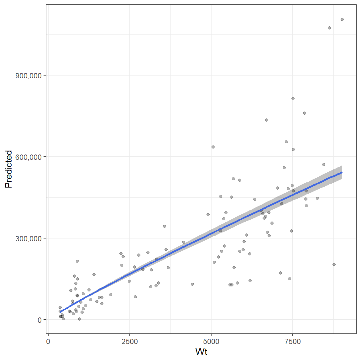
This function can also automatically estimate batch fecundity by allowing some of the parameters to be fixed. This is performed using the fixed.pars argument which requires a vector with the listed parameters to be fixed. Determining whether this is necessary is done by running the function and returning the parameters.
Estimate_Batch_Fecundity(fecundity_data_GonardFrWT,
                         start_pars = parameters,
                         return.parameters = TRUE)
#>   Parameter         Val         var
#> 1     alpha 137.2393943 68.30173197
#> 2      beta   0.9097546  0.05950147
#> 3    Sigma0  11.6937861 12.94874258
#> 4    Sigma1   0.7412575  0.08999572
For South Australian Snapper, the variances of the alpha and Sigma0 parameters are clearly overestimated. The function fixes this by running the model twice; once with all four parameters estimated and then again with the fixed parameters (ones which were estimated correctly the first time) held at their estimates from the first model. For example:
Estimate_Batch_Fecundity(fecundity_data_GonardFrWT,
                         start_pars = parameters,
                         fixed.pars = c("Sigma1", "beta"),
                         return.parameters = TRUE)
#>   Parameter         Val        var
#> 1     alpha 137.2393943 6.27413417
#> 2      beta   0.9097547 0.05950243
#> 3    Sigma0  11.6937861 0.88238412
#> 4    Sigma1   0.7412574 0.08999186
Weight The parameters for W and F are determined using a single function called Estimate_mean_W_F(). This function requires:
- A dataframe of
weight.datawhich will be used to estimate W and estimate F based on the fecundity-at-weight relationship. - A character string for
TotalWtindicating the variable name for Total weight in grams. This will be used to estimate W. - A character string for
GonadFrWtindicating the variable name for gonad free weight in grams. This will be used to estimate F for each weight. If gonad free weight is not available, then this argument can be leftNULLwhich will prompt the function to estimate fecundity based on total weight instead. NOTE: If total weight is used to determine F then total weight should be used in return batch fecundity parameters fromEstimate_Batch_Fecundity()as well - A dataframe of batch fecundity relationship parameters from
Estimate_Batch_Fecundity()withreturn.parameters = TRUE. The object returned from this call can be directly provided toEstimate_mean_W_F().
As with other functions, providng Time/Region variable names will group the results either spationally, temporally or both. Here a Region grouping is applied.
# data structure
head(Wt_data)
#>   Year Region CFL Tot_WT..kgs. Tot_Wt..g. Sex Gonad.maturity Gonad.Wt Tot.Wt
#> 1 2018   NGSV 432        1.544       1544   F              3       70   1544
#> 2 2018   NGSV 485        2.374       2374   F              3      136   2374
#> 3 2018   NGSV 433        1.522       1522   F              3       42   1522
#> 4 2018   NGSV 435        1.592       1592   F              3       32   1592
#> 5 2018   NGSV 384        1.152       1152   F              3       18   1152
#> 6 2018   NGSV 411        1.410       1410   F              3       32   1410
#>   Gonad_free_Wt
#> 1          1474
#> 2          2238
#> 3          1480
#> 4          1560
#> 5          1134
#> 6          1378

# Estimate mean W and mean F using total weight and gonad free weight, respectively.
F_W_results <- Estimate_mean_W_F(weight.data = Wt_data,
                              TotalWt = "Tot.Wt",
                              GonadFrWt = "Gonad_free_Wt",
                              Region = "Region",
                              parameters = Batch_fec_pars)
F_W_results
#>   Region    Mean_W     var_W    Mean_F     var_F
#> 1   NGSV 1166.5000 31129.417  80851.33 232341687
#> 2    SSG  507.5385  2063.444  38843.36  68653855
#> 3    NSG  849.7143  8405.862  62139.26 130449923
#> 4   SGSV 2440.0174  9619.222 157896.40  60117190
Spawning Area (A)
Spawning area is the only DEPM parameter that is not estimated in this package as this is typically done using GIS methods. However, the Spawning area object can be created manually by taking another parameter object (P0, S or R are good choices) and using its Time/Region groupings to create new object. As this example has one survey from 4 regions in a single year, only the Region variable needs to be carried across. A new variable can then be added with the location in the correct order in that column. Spawning Area is a precise quantity and therefore does not require a variance. Note that spawning area must be in metres squared.
# Get Time/region combos from the P0 object
Area <- select(P0_results, Region)

Area$A <- c(2822201039, #NGSV
            1884895030, # NSG
            2285649237, # SGSV
            3239913469) # SSG

head(Area)
#> # A tibble: 4 x 2
#>   Region          A
#>   <fct>       <dbl>
#> 1 NGSV   2822201039
#> 2 NSG    1884895030
#> 3 SGSV   2285649237
#> 4 SSG    3239913469
Combining parameters as inputs for biomass estimation
With all of the parameters now available to calculate spawning stock biomass, these now need to be combined into a dataset that can be input into the Estimate_DEPM_Biomass() function. For the DEPM approach, two objects are needed:
Combining parameter estimates
A dataframe of all of the parameter estimates can be assembled using combine_estimates() where each of the parameter objects are provided as arguments.
Adults_pars <- combine_estimates(P0 = P0_results, R = sex_ratio_results, S = Spawn_results, A = Area, W_F = F_W_results)
#> Joining, by = "Region"Joining, by = "Region"Joining, by = "Region"
Adults_pars
#> # A tibble: 4 x 8
#>   Region    P0     Z     R          A     S     W      .F
#>   <fct>  <dbl> <dbl> <dbl>      <dbl> <dbl> <dbl>   <dbl>
#> 1 NGSV   2.03    0.4 0.448 2822201039 0.722 1166.  80851.
#> 2 NSG    0.947   0.4 0.337 1884895030 0.722  850.  62139.
#> 3 SGSV   0.527   0.4 0.394 2285649237 0.722 2440. 157896.
#> 4 SSG    0.725   0.4 0.574 3239913469 0.722  508.  38843.
Where a parameter is estimated as time invariant, it will be automatically allocated to all of the Region or Time groupings applied for the other parameters. Here this occurs for S. However, if a particular parameter is missing in one instance but is not time invariant, it will not be carried over and NA will be returned. In this situation, it will need to be inserted manually. For example, lets pretend that R is missing for “SSG”:
Combining parameter variances
Variance estimates are needed by Estimate_DEPM_Biomass() in order to determine the precision of the biomass estimates. These are provided in the same fashion as the parameter estimates using combine_variances().
Adults_vars <- combine_variances(P0_results, R = sex_ratio_results, S = Spawn_results, W_F = F_W_results)
#> Joining, by = "Region"Joining, by = "Region"
Adults_vars
#> # A tibble: 4 x 7
#>   Region     P0     Z        R       S      W         .F
#>   <fct>   <dbl> <dbl>    <dbl>   <dbl>  <dbl>      <dbl>
#> 1 NGSV   0.391    0.4 0.00952  0.00298 31129. 232341687.
#> 2 NSG    0.218    0.4 0.000714 0.00298  8406. 130449923.
#> 3 SGSV   0.129    0.4 0.00117  0.00298  9619.  60117190.
#> 4 SSG    0.0849   0.4 0.00185  0.00298  2063.  68653855.
The same manual insertions can be performed on this object:
Spawning Stock Biomass Estimation
All of the hard work is done once all of the parameters and their variances have been estimated and organised. The final step is to combine them using Estimate_DEPM_Biomass(). This function requires each of these objects and will return a list of results which include the spawning stock biomass and total number of females.
# Estimate Biomass
Snapper_biomass_results <- Estimate_DEPM_Biomass(adult.pars = Adults_pars,
                                          adult.vars = Adults_vars)
# a list of two outputs is returned
Snapper_biomass_results$Biomass # biomass in kgs
#>   Region   Z   Biomass        SD
#> 1   NGSV 0.4 255865.89 116146.47
#> 2    NSG 0.4 100289.06  54941.25
#> 3   SGSV 0.4  65373.53  45453.08
#> 4    SSG 0.4  74034.41  35203.09
Snapper_biomass_results$Nfem # number of females
#>   Region   Z     Nfem        SD
#> 1   NGSV 0.4 98236.78 36190.250
#> 2    NSG 0.4 39769.07 21125.853
#> 3   SGSV 0.4 10555.32  7269.309
#> 4    SSG 0.4 83749.33 38604.596
The list of dataframes returned from the function can then be saved and used for plotting
# Create new objects
Snapper_biomass <- Snapper_biomass_results$Biomass
Snapper_Nfem <- Snapper_biomass_results$Nfem
Plot biomass with SD
ggplot(Snapper_biomass, aes(Region,Biomass,
                            ymin = Biomass - SD,
                            ymax = Biomass + SD))+
  geom_crossbar(fill = "royalblue", alpha = .8)+
  expand_limits(y = 0)+
  scale_y_continuous(name = "Biomass (kg)", labels = scales::comma, breaks = scales::pretty_breaks(5))+
  theme_bw()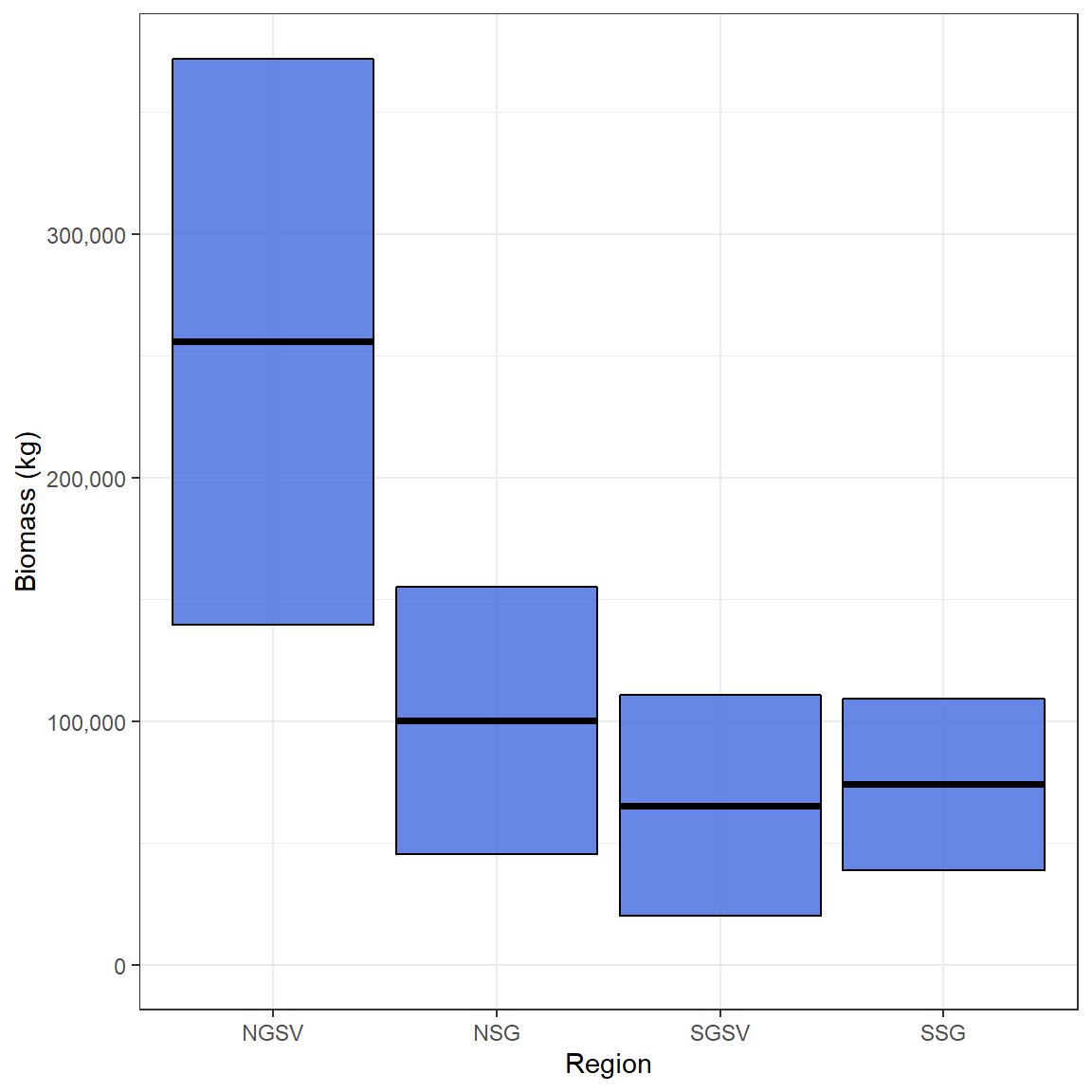
Plot total number of females
ggplot(Snapper_Nfem, aes(Region,Nfem,
                            ymin = Nfem - SD,
                            ymax = Nfem + SD))+
  geom_crossbar(fill = "purple", alpha = .8)+
  expand_limits(y = 0)+
  scale_y_continuous(name = "Number of females", labels = scales::comma, breaks = scales::pretty_breaks(5))+
  theme_bw()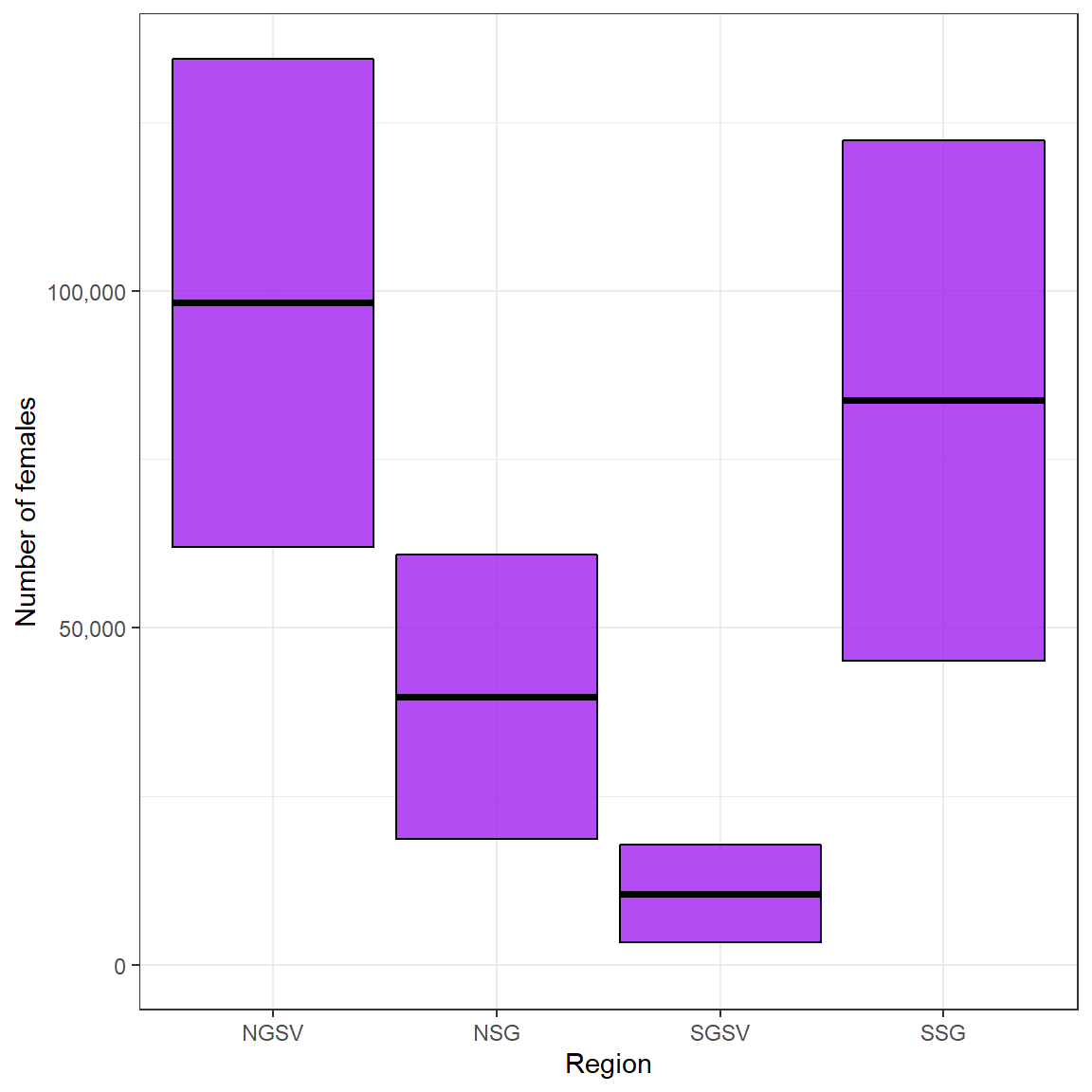
Testing assumptions for pre-specified egg mortality (Z)
As the \(P_{0}\) estimation methods in this package require a specified level of egg mortality (Z), it is sensible to test the sensitivities of the \(P_{0}\) estimates, as well as the DEPMWt results to different Z values. Testing different values of Z can be done by passing a vector of values to the z argument of Estimate_P0():
Multi_Z_P0_results <- Estimate_P0(data = egg_data,
                          site = "Site",
                          Region = "Region",
                          Z = c(.2, .4, .6))
This will return a different \(P_{0}\) estimate for each value of Z for each Time/Region grouping:
Multi_Z_P0_results
#>    Region        P0      P0_se   Z
#> 1    NGSV 1.7972317 0.35215150 0.2
#> 2     NSG 0.8400430 0.19454626 0.2
#> 3    SGSV 0.4600852 0.11248190 0.2
#> 4     SSG 0.6294788 0.07419926 0.2
#> 5    NGSV 2.0333120 0.39057148 0.4
#> 6     NSG 0.9472290 0.21775974 0.4
#> 7    SGSV 0.5268231 0.12938292 0.4
#> 8     SSG 0.7254297 0.08486910 0.4
#> 9    NGSV 2.3084189 0.43464390 0.6
#> 10    NSG 1.0709549 0.24423117 0.6
#> 11   SGSV 0.6061931 0.15043110 0.6
#> 12    SSG 0.8390163 0.09755602 0.6
For South Australian Snapper, the resulting \(P_{0}\) estimates are very similar.
Multi_Z_P0_results$Z <- as.factor(Multi_Z_P0_results$Z) # convert Z to a factor for easy plotting

ggplot(Multi_Z_P0_results, aes(Z, P0, ymin = P0 - P0_se, ymax = P0 + P0_se, fill = Z))+
  geom_crossbar()+
  facet_wrap(~Region, ncol = 2, scales = "free")+
  scale_fill_viridis_d()+
  theme_bw()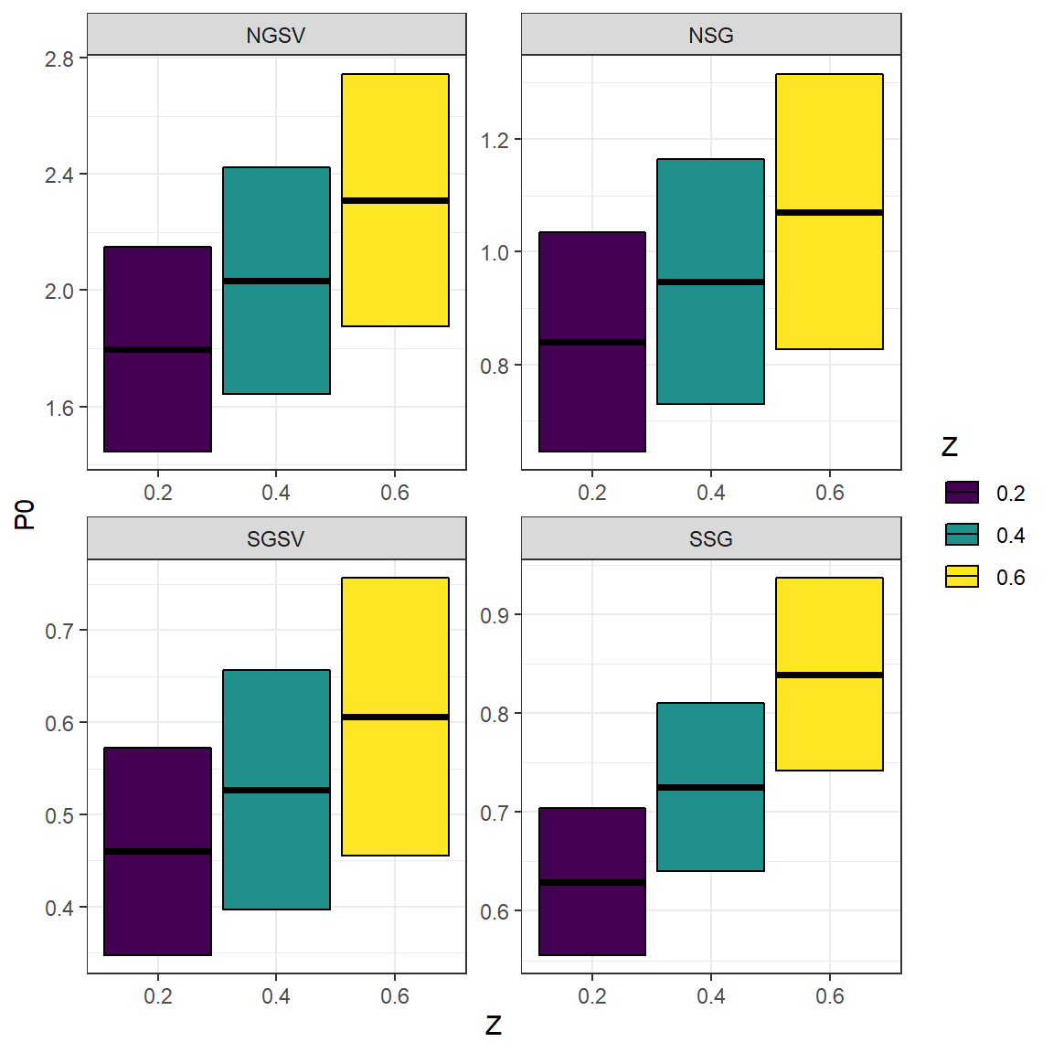
An object from Estimate_P0() with multiple Zs can be included in the biomass estimation procedure in the same manner as before. When multiple Zs are provided to combine_estimates() and combine_variances() they are treated as groupings and all other parameters will be aligned with them. When creating an object for spawning area A, care must be taken to only have unique Time/Region groupings. Using an object from Estimate_P0() with multiple Zs can erroneously add duplicates if you’re not careful. This will cause error messages.
# Make sure that Area has unique Time/Region breakdowns (Only Region used in this example)
Area <- data.frame(Region = unique(Multi_Z_P0_results$Region))

Area$A <- c(2822201039, #NGSV
            1884895030, # NSG
            2285649237, # SGSV
            3239913469) # SSG


Multi_Z_adult_pars <- combine_estimates(P0 = Multi_Z_P0_results, R = sex_ratio_results, S = Spawn_results, A = Area, W_F = F_W_results)
#> Joining, by = "Region"Joining, by = "Region"Joining, by = "Region"

Multi_Z_adult_vars <- combine_variances(P0 = Multi_Z_P0_results, R = sex_ratio_results, S = Spawn_results, W_F = F_W_results)
#> Joining, by = "Region"Joining, by = "Region"
A new object with Z as a grouping will now be produced which can be passed to the biomass estimation function.
Multi_Z_adult_pars
#>    Region        P0   Z         R          A        S         W        .F
#> 1    NGSV 1.7972317 0.2 0.4478643 2822201039 0.722488 1166.5000  80851.33
#> 2     NSG 0.8400430 0.2 0.3369494 1884895030 0.722488  849.7143  62139.26
#> 3    SGSV 0.4600852 0.2 0.3939694 2285649237 0.722488 2440.0174 157896.40
#> 4     SSG 0.6294788 0.2 0.5741385 3239913469 0.722488  507.5385  38843.36
#> 5    NGSV 2.0333120 0.4 0.4478643 2822201039 0.722488 1166.5000  80851.33
#> 6     NSG 0.9472290 0.4 0.3369494 1884895030 0.722488  849.7143  62139.26
#> 7    SGSV 0.5268231 0.4 0.3939694 2285649237 0.722488 2440.0174 157896.40
#> 8     SSG 0.7254297 0.4 0.5741385 3239913469 0.722488  507.5385  38843.36
#> 9    NGSV 2.3084189 0.6 0.4478643 2822201039 0.722488 1166.5000  80851.33
#> 10    NSG 1.0709549 0.6 0.3369494 1884895030 0.722488  849.7143  62139.26
#> 11   SGSV 0.6061931 0.6 0.3939694 2285649237 0.722488 2440.0174 157896.40
#> 12    SSG 0.8390163 0.6 0.5741385 3239913469 0.722488  507.5385  38843.36

# Estimate Biomass
Snapper_biomass_results <- Estimate_DEPM_Biomass(adult.pars = Multi_Z_adult_pars,
                                          adult.vars = Multi_Z_adult_vars)


# Create new objects
Snapper_biomass <- Snapper_biomass_results$Biomass
Snapper_Nfem <- Snapper_biomass_results$Nfem
These results can then be examined to determine how biomass is influenced by the specification of Z.
Snapper_biomass$Z <- as.factor(Snapper_biomass$Z) # convert Z to a factor for easy plotting

ggplot(Snapper_biomass, aes(Z,Biomass, fill = Z,
                            ymin = Biomass - SD,
                            ymax = Biomass + SD))+
  geom_crossbar( alpha = .8)+
  facet_wrap(~Region, ncol =2)+
  scale_fill_viridis_d()+
  expand_limits(y = 0)+
  scale_y_continuous(name = "Biomass (kg)", labels = scales::comma, breaks = scales::pretty_breaks(5))+
  theme_bw()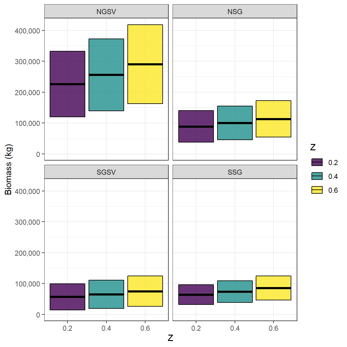
References
McGarvey, R., Steer, M. A., Smart, J. J., Matthews, D. J. and Matthews, J. M.(in review). Generalizing the Parker model equation of DEPM: incorporating size dependence of population numbers and batch fecundity
McGarvey, R., Steer, M.A., Matthews, J.M., Ward, T.M. (2018). A stage-based estimator of daily egg production. ICES J. Mar. Sci. 75(5), 1638-1646.